Tutorial: Solving Continuous Domains

Tutorials > Solving Continuous Domains > Part 3

Tutorial Contents

Solving Lunar Lander with SARSA(λ)

In our final example of this tutorial we will solve a simplified Lunar Lander domain using gradient descent Sarsa Lambda and Tile coding basis functions. The Lunar Lander domain is a simplified version of the classic 1979 Atari arcade game by the same name. In this domain the agent pilots a ship that must take off from the ground and land on a landing pad. The agent can either use a strong rocket thruster to push the ship in the direction the ship is facing, use a weak rocket thruster that is equal magnitude to the force of gravity, rotate clockwise or counterclockwise, or coast. The agent will receive a large reward for landing on the landing pad, a large negative reward for colliding with the ground or an obstacle, and a small negative reward for all other transitions.

As with the previous examples, let us begin by making a method for this example (LLSARSA) and instantiating a Lunar Lander domain, task, and initial state.

public static void LLSARSA(){

	LunarLanderDomain lld = new LunarLanderDomain();
	OOSADomain domain = lld.generateDomain();

	LLState s = new LLState(new LLAgent(5, 0, 0), new LLBlock.LLPad(75, 95, 0, 10, "pad"));
}

Most of this code should be fairly self explanatory. Using a default construct for LunarLanderDomain and not setting anything else with it will use default parameters for the domain (but you can change various properties such as the force of gravity, thrust, etc.). The default reward function returns +1000 for landing, -100 for collisions, and -1 for regular transitions (you can also change the reward function for the domain in the usual ways). The terminal function sets all states in which the ship has landed on the landing pad as terminal states. The initial state sets the agent at location 5, 0, with facing up, and with zero velocity (the 0 velocity is implict with the 3 argument constructor); and sets a goal landing pad rectange spanning 75-90 along the x dimension and 0-10 along the y dimension. This will create an initial state that looks like the below (as visualized in BURLAP).

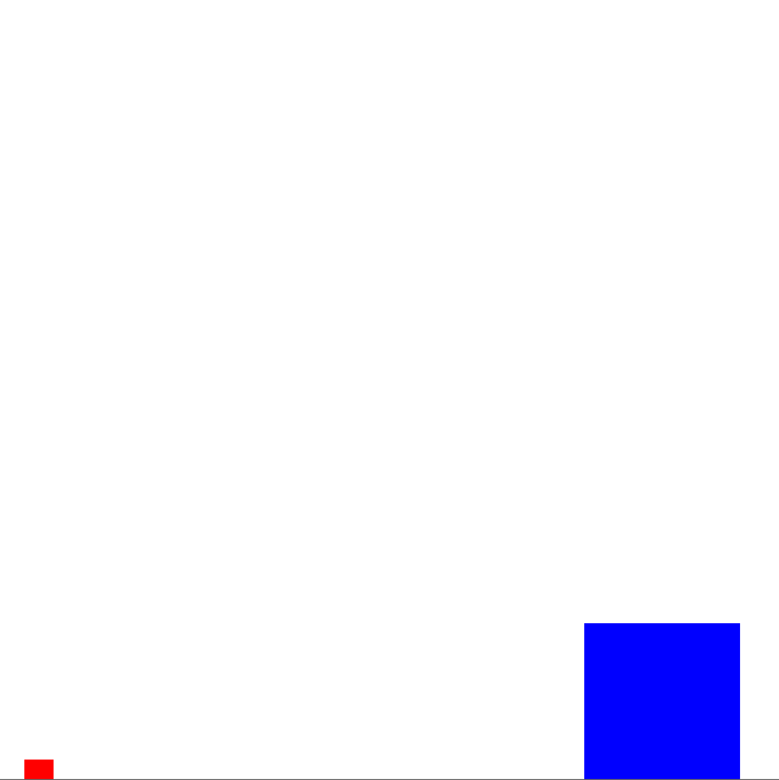
The initial stated used in Lunar Lander. The red box is the ship, the blue box the landing pad.

We're going to solve this problem with gradient descent SARSA(λ), which is a learning algorithm that behaves much like conventional tabular SARSA(λ) (discussed in previous tutorials), except it learns an approximation of the value function, much like LSPI. Unlike LSPI, gradient descent SARSA(λ) does not need to use a linear approximator; however, in practice it is usually a good idea to use a linear approximator because there are much stronger learning convergence guarantees with linear approximators. When using a linear approximator, it is a good idea then to use some kind of basis functions. Like in the LSPI example, we could use the same Fourier basis or radial basis functions for gradient descent SARSA(λ). However, this time we'll use a different basis function: Tile coding.

Tile coding creates a set of features by generating multiple tilings over the state space. Each tile represents a features and that feature is "on" if the state falls within that tile.

Tile coding in detail

Tile coding address learning in continuous domains in an only slightly more complex way than merely discretizing the state space, yet also diminishes the aliasing effects that discretization can incur. To describe how it works, lets start by thinking about how a state discretization can be used to create a set of binary basis functions. First imagine a discretization of the state space as a process that creates large bins, or tiles, across the entire state space. We'll let each tile represent a different binary basis function. For a given input continuous state, all basis functions return a value of 0, except the function for the tile in which the continuous state is contained, which will return a value of 1. By then estimating a linear function over these features, we generalize the observed rewards and transitions for one state to all states that are contained in the same tile. The larger the tiles we use, the larger the generalization. A disadvantage of using such a simple discretization is that it produces aliasing effects. That is, two states may be very similar but reside on opposite sides of the edge of a tile, which results in none of their experience being shared, despite the fact that they are similar and do share experiences with other states that are more distant but happen to be in the same tile.

Tile coding diminishes this aliasing effect by instead creating multiple offset tilings over the state space and creating a basis function for each tile in each of the tilings. If there are n tilings, then any given input state will have n basis functions with a value 1 (one for each active tile in each tiling). Because the tilings are offset from each other, two states may be contained in the same tile of one tiling, but in different tiles for a different tiling. As a consequence, experience generalization still occurs between states in the same tiling, but the differences between different tilings regains specificity and removes aliasing effects. For more information on tile coding with some good illustrations, we recommend the Generalization and Function Approximation chapter in the book Reinforcement Learning: An Introduction, by Sutton and Barto. An online version of the chapter can be found here.

An advantage of using tile coding is that you only need to store weight values in the fitted linear function for tiles that are associated with states that the agent has experienced thus far (the basis function for all other tiles would return a value of zero and therefore contribute nothing to the value function approximation). Morever, when computing the value for a given input state, you only need to add the weights for the active tiles and can ignore all other tiles; that is, tile coding can be represented sparsely.

Lets continue our code implementation by instantiating a TileCodingFeatures object (and implementation of SparseStateFeatures) and define the tiling of our state space. To implement tile coding basis functions, we will need to decide on the number of tilings that we use and the width of each tile along each variable. In this case, we will use 5 tilings with a width for each variable that produces 10 tiles along each variable range. We will limit this tiling to the Lunar Lander ship variables values and ignore variables for the landing pad. Since the agent's ship is defined by 5 variables (x position, y position, x velocity, y velocity, and rotation angle from the vertical axis), this will produce 5 tilings that each define at most 10^5 tiles (since tiling coding can be represtently sparsely though, we don't necessarily have to store weights for all tiles if the agent never visits them!) To do so, add the below code.

ConcatenatedObjectFeatures inputFeatures = new ConcatenatedObjectFeatures()
				.addObjectVectorizion(LunarLanderDomain.CLASS_AGENT, new NumericVariableFeatures());

int nTilings = 5;
double resolution = 10.;

double xWidth = (lld.getXmax() - lld.getXmin()) / resolution;
double yWidth = (lld.getYmax() - lld.getYmin()) / resolution;
double velocityWidth = 2 * lld.getVmax() / resolution;
double angleWidth = 2 * lld.getAngmax() / resolution;



TileCodingFeatures tilecoding = new TileCodingFeatures(inputFeatures);
tilecoding.addTilingsForAllDimensionsWithWidths(
		new double []{xWidth, yWidth, velocityWidth, velocityWidth, angleWidth},
		nTilings,
		TilingArrangement.RANDOM_JITTER);

To specify our tilings on the state variables, we will first want to convert our states into a variable vector. Lunar lander states are OO-MDP representations, so to vectorize the state, we use the ConcatenatedObjectFeatures class. This class lets us specify a variable vectorization for certain object classes, and then produce a state variable vector by concatenating the vectors for each object of those classes. In this case, we set it to create a state vector consisting of just the agent object class, and the agent object class is vectorized by assuming each of its variables are numeric and filling them out into an array (functionality provided by the NumericVariableFeatures class, a DesneStateFeatures implementation).

Next we create some local variable for specifying our tiling configuration. We choose to 5 tilings and we set the "resolution" to be 10; which is how many tiles will span a variable dimension. Then, we set the width of the tiles along each dimension by dividing the range of the variable by our resolution. Our LunarLanderDomain object has methods for getting these variable range values.

Finally, we instantiate our TileCodingFeatures, an implementation of SparseStateFeatures, which means it provides a method that will return a list of of any non-zero state features for a given state input. We give it the state vectorization we're using for states, and provide it tile widths along each of those dimensions, tell it to create 5 tilings along that space, and that those 5 tilings should be randomly offset from each other. If you wanted, you could also add additional tilings that operated on different sets of state variables--an advanced functionality of tile coding.

Now that we have the TileCodingFeatures set up, we can create a linear value function approximator for it and pass it along to gradient descent SARSA(λ).

double defaultQ = 0.5;
DifferentiableStateActionValue vfa = tilecoding.generateVFA(defaultQ/nTilings);
GradientDescentSarsaLam agent = new GradientDescentSarsaLam(domain, 0.99, vfa, 0.02, 0.5);

SARSA lambda, like LSPI, requires state-action features, and TileCoding only provides state features. However, by default the generateVFA method of TileCoding will produce a function approximator that will cross product its features with the actions, if it is used for state-action value function approximation (it also implements DifferentiableStateValue to provide state value function approximation).

Note that to set the initial default Q-values to be predicted to 0.5, we set the value of each feature weight to 0.5 divided by the number of tilings. We divide the desired initial Q-value (0.5) by the number of tilings (5), because for any given state there will only be n features with a value of 1 and the rest 0, where n is the number of tilings. Therefore, if the initial weight value for all those features is 0.5/5, the linear estimate will predict our desired initial Q-value: 0.5. We also set the learning rate for gradient descent SARSA(λ) to 0.02 (in general, you should decrease the learning rate as the number of features increases), and set λ to 0.5.

With gradient descent SARSA(λ) instantiated, we can run learning episodes wtih an Environment just like we do for typical SARSA(λ). Lets create a SimulatedEnvironment, run learning for 5000 episodes, and then visualize the results with an EpisodeSequenceVisualizer.

SimulatedEnvironment env = new SimulatedEnvironment(domain, s);
List episodes = new ArrayList();
for(int i = 0; i < 5000; i++){
	Episode ea = agent.runLearningEpisode(env);
	episodes.add(ea);
	System.out.println(i + ": " + ea.maxTimeStep());
	env.resetEnvironment();
}

Visualizer v = LLVisualizer.getVisualizer(lld.getPhysParams());
new EpisodeSequenceVisualizer(v, domain, episodes);

If you now point your main method to LLSARSA() and run it, you should initially see a bunch of text after each episode stating how long the learning episode lasted followed by the EpisodeSequenceVisualizerGUI, which should look something like the below.

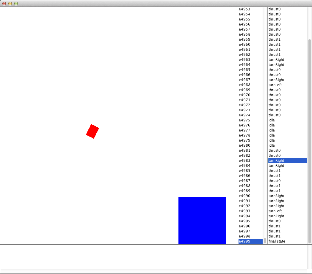
The EpisodeSequenceVisualizer GUI showing the learning results on Lunar Lander

You should find that as more learning episodes are performed, the agent becomes progressively better at piloting to the landing pad.

That concludes all of our examples for this tutorial! Closing remarks and the full code we created can be found on the next page.

Next Part