Tutorial: Basic Planning and Learning

Tutorials (v1) > Basic Planning and Learning > Part 5

Tutorial Contents

Live Visualization

Although we showed how to visualize learning or planning results after they had been performed, sometimes when setting up a new problem and experiment it is useful to watch what is happening immediately. In this part of the tutorial we show how to set up a live visualization of learning algorithms or planning algorithms that operate by trying actions in the world (more on that in a bit). To present a live visualization we make use of the ActionObserver interface. Objects that adhere to the ActionObserver interface can be passed to Action objects in a domain. Whenever the action is executed in a state, the action will automatically inform the the observer of the state, action, nextState event before returning the result to the code that executed the action. You can use this interface to do any kind of analysis you want, but in this tutorial we will show how we can use a built in VisualActionObserver class to watch learning or planning unfold as it is happening.

Note

The action observer class only works when the performAction method is called on an action. This means that ActionObservers will work for learning algorithms, in which the agent must sequentially interact with the world, and planning algorithms that try executions of actions. However, you cannot use an ActionObserver to intercept what a planning algorithm like VI does, because VI uses the Action transition dynamics to perform planning, rather than taking actions in states.

It is worth noting further that the forward search deterministic planning algorithms do work with ActionObserver objects, because the planners operate by applying actions to states. This may have some interesting visualizations, since forward search planning algorithms like A* will hop around the state space.

To use our VisualActionObserver, first add the necessary import.

import burlap.oomdp.singleagent.common.VisualActionObserver;

Then, we can modify our constructor by adding the following lines to then end of it:

VisualActionObserver observer = new VisualActionObserver(domain, 
			GridWorldVisualizer.getVisualizer(gwdg.getMap()));
((SADomain)this.domain).setActionObserverForAllAction(observer);
observer.initGUI();

The first line creates a VisualActionObserver for visualizing our domain with a provided domain state visualizer (we use the same state visualizer that we used for our EpisodeSequenceVisualizer). The second line tells the domain to add this observer for all actions in the domain. We could have alternatively only added the observer to specific actions that we wanted to observe, but since we want to watch everything that happens, we added to all actions. The last line will cause a GUI showing the viewer to appear.

Now that the observer is set up, try running one of the learning algorithms that we set up previously. You should have a visualizer pop up showing what the agent is doing at each step of learning!

Note

By default, the VisualActionObserver will render frames at about 60FPS. You can modify this rate with the setFrameDelay(long delay) method, which takes as an argument the number of ms that must pass for the rendering of an event and before the next action can be taken. Note that this delay also places a cap on the speed at which learning occurs. Typically, learning in BURLAP occurs at speeds orders of magnitude faster than 60FPS, so using the visual observer will slow down your algorithm considerably. Nevertheless, it is often useful as a way to confirm that your experiment is working as planned.

Value Function and Policy Visualization

While visualizing the agent in the state space is useful, in this next section, we will show how to visualize the value function that is estimated from value function estimating planning or learning algorithms, along with the corresponding policy. In particularly we will show how to visualize it for ValueIteration, but you could do the same with Q-Learning, or any planning/learning algorithm that implements the QComputablePlanner interface.

The first step will be to add our necessary imports.

import java.awt.Color;
import java.util.List;

import burlap.behavior.singleagent.auxiliary.StateReachability;
import burlap.behavior.singleagent.auxiliary.valuefunctionvis.ValueFunctionVisualizerGUI;
import burlap.behavior.singleagent.auxiliary.valuefunctionvis.common.ArrowActionGlyph;

Then we will define a new method in our class to perform this visualization. The method will take a QComputablePlanner object and a policy for it that we wish to visualize.

public void valueFunctionVisualize(QComputablePlanner planner, Policy p){
		List <State> allStates = StateReachability.getReachableStates(initialState, 
			(SADomain)domain, hashingFactory);
		LandmarkColorBlendInterpolation rb = new LandmarkColorBlendInterpolation();
		rb.addNextLandMark(0., Color.RED);
		rb.addNextLandMark(1., Color.BLUE);
		
		StateValuePainter2D svp = new StateValuePainter2D(rb);
		svp.setXYAttByObjectClass(GridWorldDomain.CLASSAGENT, GridWorldDomain.ATTX, 
			GridWorldDomain.CLASSAGENT, GridWorldDomain.ATTY);
		
		PolicyGlyphPainter2D spp = new PolicyGlyphPainter2D();
		spp.setXYAttByObjectClass(GridWorldDomain.CLASSAGENT, GridWorldDomain.ATTX, 
			GridWorldDomain.CLASSAGENT, GridWorldDomain.ATTY);
		spp.setActionNameGlyphPainter(GridWorldDomain.ACTIONNORTH, new ArrowActionGlyph(0));
		spp.setActionNameGlyphPainter(GridWorldDomain.ACTIONSOUTH, new ArrowActionGlyph(1));
		spp.setActionNameGlyphPainter(GridWorldDomain.ACTIONEAST, new ArrowActionGlyph(2));
		spp.setActionNameGlyphPainter(GridWorldDomain.ACTIONWEST, new ArrowActionGlyph(3));
		spp.setRenderStyle(PolicyGlyphRenderStyle.DISTSCALED);
		
		ValueFunctionVisualizerGUI gui = new ValueFunctionVisualizerGUI(allStates, svp, planner);
		gui.setSpp(spp);
		gui.setPolicy(p);
		gui.setBgColor(Color.GRAY);
		gui.initGUI();
}

In the first line, we first define a set of states for which we want the value function and policy visualized. In our example, we'd like to simply visualize all the states in our domain, which means we want to find all the states in our domain. We can do this by using the StateReachability tool, which takes as input an initial state, a single agent domain, a hashing factory to identify and perform equality checks between states, and returns a list of all states that are reachable from the provided initial state. Note that the GridWorld domain is an instance of the single agent domain class (SADomain), so we can type cast it in this way (the alternative is a domain for stochastic games, which involve multiple simultaneously acting agents).

For our visualization we're going to render the value of a state with a color between red (for low values) and blue (for high values). The LandmarkColorBlendInterpolation class can be used to do this, which you can note has a landmark added first for red and then for blue. If we wanted to render across more colors (like a rainbow scale) we could have continued adding more colors.

Following our color blend definition, we then create a 2D value function visualizer, which requires a color blend object (which we just created) to define the color shown for the value of states. This class also requires it to be told which attributes for which class should be used to determine the x and y coordinates to render each state. In this case, we want to use the agent's X and Y attributes to determine the location on a screen that a state is rendered.

We could stop here and only visualize the value function, but it may also be useful to visualize the policy derived. In this case, we will render the policy using a PolicyGlyphPainter2D. Similar to the value function painter we defined above, this class needs to be told which attributes for which class correspond to where a state's policy will be rendered on the screen; again we use the agent X and Y attributes. This class also wants to be told which glyph to paint for each action. We will use the prebuilt ArrowActionGlyph class, which takes as input a direction for an arrow with 0,1,2, and 3 corresponding to a north, south, east, and west arrow glyph, respectively. Finally, The PolicyGlyphPainter2D class also needs to be told how to render a policy. That is, some policies are stochastic, which requires the painter to determine how to render each glyph for each action based on the probability of that action being taken by the agent. The PolicyGlyphRenderStyle.MAXACTION specification tells the painter to only render the glyph for the action with the maximum probability of being selected; if there are ties for the max, then all actions that tied for max will be rendered. See the class documentation for the other policy render modes.

The final lines of this method create our ValueFunctionVisualizerGUI, which takes the states to render, the object that defines how the value function is rendered, and the QComputablePlanner which specifies the value function. The policy and policy painter are optional, so they are passed as arguments through the subsequent method calls. We also set the background color of the canvas to be grey and then launch the GUI.

Try calling this method from the VI method we created earlier, passing it the VI object and its policy, and see what happens.

//visualize the value function and policy
this.valueFunctionVisualize((QComputablePlanner)planner, p);

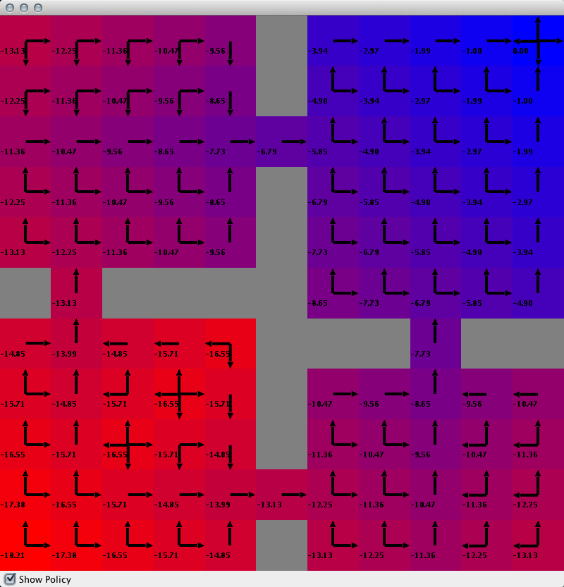
You may also want to disable in main the method that activates the offline EpisodeSequenceVisualizer, so that you do not have two different GUIs floating around. You should get a GUI with colors in each cell of the of the world representing the value function in that state as well as the numeric value written in text (the text rendering can be disable if desired, or have its font properties and position manipulated). Additionally, if you check the "Show Policy" check box at the bottom of the window you'll see arrows indicating the policy. The below image should resemble what you see.

Next Part