Tutorial: Building a Domain
Tutorials > Building a Domain > Part 1
- Introduction
- Markov Decision Process
- OO-MDPs
- BURLAP OO-MDP Java Class Overview
- Defining GridWorld Object Classes
- Defining GridWorld Actions
- Defining Propositional Functions
- Testing the Domain
- The Components of a Visualizer
- Implementing the Painters
- Reward Functions and Terminal Functions
- Conclusions
- Final Code
You are viewing the tutorial for BURLAP 2; if you'd like the BURLAP version 1 tutorial, go here.
Introduction
This tutorial will cover three topics. First, we will discuss Markov Decision Processes (MDPs) and more specifically, Object-oriented MDPs (OO-MDPs): the decision making process that BURLAP uses to express single agent domains and decision making problems; then we will discuss how BURLAP implements that OO-MDPs. Finally, we will cover how to create a domain, so that the planning and learning algorithms in BURLAP can be used on it, as well as how to visualize it, which is useful for testing and reviewing results.
Other Problem Types
Beyond MDPs, BURLAP also supports stochastic games and partially observable MDPs, but a discussion of those problem types will be left for a different tutorial and many of the core elements of the OO-MDP code that BURLAP uses is reused with the other problem types.
If you are already familiar with MDPs or OO-MDPs, or just want to get down to coding, feel free to skip the first sections that discuss their mathematical description.
For more information on how to use planning and learning algorithms on the OO-MDP domains that you create or that are already in BURLAP, see the Basic Planning and Learning tutorial.
Markov Decision Process
To define worlds in which an agent can plan or learn, BURLAP uses the object-oriented Markov Decision Process (OO-MDP) formalism, which is an extension of the classic Markov Decision Process (MDP) formalism. An MDP provides a formal definition of a world, how it works, and how the agent who will be making decisions interacts with the world in a series of discrete time steps. In this tutorial we will formalize a grid world as an MDP. A grid world is a 2D world in which an agent can move north, south, east or west by one unit, provided there are no walls in the way. The below image shows a simple grid world with the agent's position represented by a gray circle and walls of the world painted black. Typically, the goal in a grid world is for the agent to navigate to some location, but there are a number of variants.
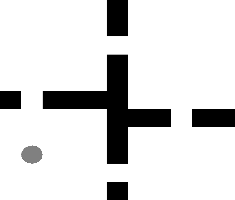
An example grid world.
To define any world and task as an MDP, we will need to break down the problem into four components: a set of possible states of the world ($S$); a set of actions that the agent can apply ($A$); a definition of how actions change the state of the world, known as the transition dynamics ($T$); and the rewards the agent receives for each of its actions ($R$), known as the reward function, which will determine what the best behavior is (that is, the agent will want to act in a way that maximizes the reward it receives).
The transition dynamics are formulated as a probabilistic function $T(s' | s, a)$, which defines the probability of the world changing to state $s'$ in the next discrete time step when the agent takes action $a$ in the current state $s$. The fact that the world can change stochastically is one of the unique properties of an MDP compared to more classic planning/decision making problems.
The reward function is defined as $R(s, a, s')$, which returns the reward received for the agent taking action $a$ in state $s$ and then transitioning to state $s'$.
Notice how both the transition dynamics and reward function are temporally independent from everything predating the most recent state and action? Requiring this level of temporal independence makes this a Markov system and is why this formalism is called a Markov decision process.
In our grid world, the set of states are the possible locations of the agent. The actions are north, south, east, and west. We will make the transition dynamics stochastic so that with high probability (0.8) the agent will move in the intended direction, and with some low probability (0.2) move in a different direction. The transition dynamics will also encode the walls of our grid world by specifying that movement that would lead into a wall will result in returning to the same state. Finally, we can define a reward function that returns a high reward when the agent reaches the top right corner of the world and zero everywhere else.
For various kinds of problems, the concept of terminal states is often useful. A terminal state is a state that once reached causes all further action of the agent to cease. This is a useful concept for defining goal-directed tasks (i.e., action stops once the agent achieves a goal), failure conditions, or any number of other reasons. In our grid world, we'll want to specify the top right corner the agent is trying to get to as a terminal state. An MDP definition does not include a specific element for specifying terminal states because they can be implicitly defined in the transition dynamics and reward function. That is, a terminal state can be encoded in an MDP by being a state in which every action causes a deterministic transition back to itself with zero reward. However, for convenience and other practical reasons, terminal states in BURLAP are specified directly with a function (more on that later).
The goal of planning or learning in an MDP is to find the behavior that maximizes the reward the agent receives over time. More formally, we'd say that the goal is to find a policy ($\pi$), that is a mapping from states in the MDP to actions that the agent takes ($\pi : S \rightarrow A$). Sometimes, the policy can also be defined as a probability distribution over action selection in each state (and BURLAP supports this represenation), but for the moment we will consider the case when it is a direct mapping from states to actions. To find the policy that maximizes the reward over time, we must first define what it means to maximize reward over time and there are a number of different temporal objectives we can imagine that change what the optimal policy is.
Perhaps the most intuitive way to define the temporal reward maximization is to maximize the the expected total future reward; that is, the best policy is the one that results in largest possible sum of all future rewards. Although this metric is sometimes appropriate, it's often problematic because it can result in policies that are evaluated to have infinite value or which do not discriminate between policies that receive the rewards more quickly. For example, in our grid world, any path the agent took to reach the top right would have a value 1 (because they all would eventually reach the goal); however, what we'd probably want instead is for the agent to prefer a policy that reaches the goal as fast as possible. Moreover, if we didn't set the top right corner to be a terminal state, the agent could simply move away from it and back into it, resulting in any policy that reaches the goal having an infinite value, which makes comparisons between different policies even more difficult!
A common alternative that is more robust is to define the objective to be to maximize the expected discounted future reward. That is, the agent is trying to maximize expected sum $$\large \sum_{t=0}^\infty \gamma^t r_t,$$ where $r_t$ is the reward received at time $t$ and $\gamma$ is the discount factor that dictates how much preference an agent has for more immediate rewards; in other words, the agent's patience. With $\gamma = 1$, the agent values distant rewards that will happen much further in the future as much as the reward the agent will receive in the next time step; therefore, $\gamma = 1$ results in the same objective of summing all future rewards together and will have the same problems previously mentioned. With $\gamma = 0$ all the agent values only the next reward and does not care about anything that happens afterwards, thereby resulting in all policies having a finite value. This setting has the inverse effect of the agent never caring about our grid world goal location unless it's one step away. However, a $\gamma$ value somewhere in between 0 and 1 often results in what we want. That is, for all values of $0 \le \gamma \lt 1$, the expected future discounted reward in an MDP when following any given policy is finite. If we set $\gamma$ to 0.99 in our grid world, the result is that the agent would want to get to the goal as fast as possible, because waiting longer would result in the eventual +1 goal reward being more heavily discounted. Although there are still other ways to define the temporal objective of an MDP, current learning and planning algorithms in BURLAP are based on using the discounted reward, with the geometric discout factor $\gamma$ left as a parameter that the user can specify.