Tutorial: Solving Continuous Domains

Tutorials (v1) > Solving Continuous Domains > Part 2

Tutorial Contents

Solving the Inverted Pendulum with Sparse Sampling

In this part of the tutorial we will be solving the Inverted Pendulum problem. There are actually a number of different versions of this problem (for other variants, see the CartPoleDomain and its parameters), but in this example we'll be using one of the more simple forms. The problem is as follows; a cart exists on an infinite track on which force can be applied to move the cart left or right on the track. On top of the cart is a pole (the inverted pendulum) and the goal is to keep the pole balanced and pointing up by using left, right, or no force actions. If the angle between the pole and the vertical axis is larger than some threshold, the task is considered to have been failed. The state is defined by a single object which is defined by the pole angle and its angular velocity. An illustration of the problem, as visualized in BURLAP, is shown below.

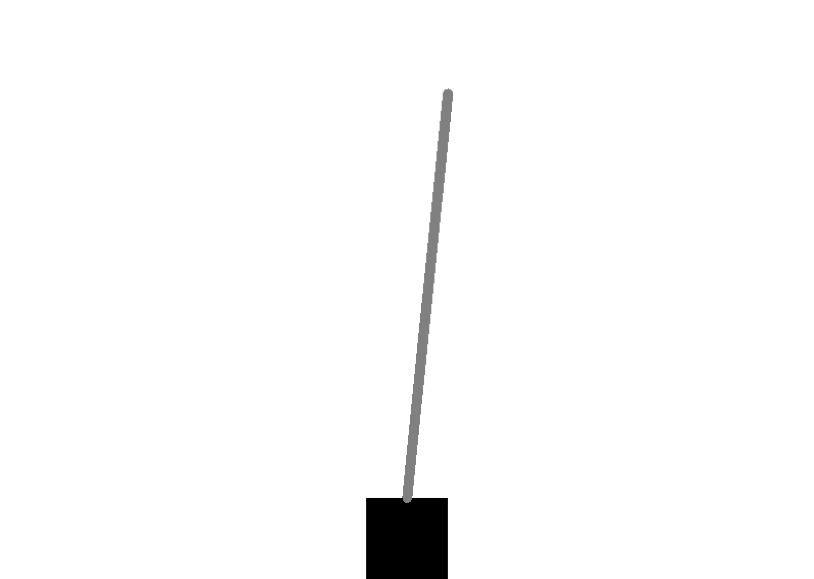
The BURLAP visualization of the Inverted Pendulum problem

We are going to solve this problem using Sparse Sampling (more on that in a moment). Let us start by making a method (IPSS) for solving this problem and filling it in with code to instantiate the InvertedPendulum domain and task.

import burlap.domain.singleagent.cartpole.InvertedPendulum;

public static void IPSS(){

	InvertedPendulum ip = new InvertedPendulum();
	ip.physParams.actionNoise = 0.;
	Domain domain = ip.generateDomain();
	RewardFunction rf = new InvertedPendulum.InvertedPendulumRewardFunction(Math.PI/8.);
	TerminalFunction tf = new InvertedPendulum.InvertedPendulumTerminalFunction(Math.PI/8.);
	State initialState = InvertedPendulum.getInitialState(domain);


}

The line "ip.physParams.actionNoise = 0.;" sets our domain to have no noise in the actions. (physParams is a data member containing all physics parameters that you can modify.) The created reward function and terminal function specify task failure conditions to be when the angle between the pole and vertical axis is greater than π/8 radians. Specifically, the agent will receive zero reward everywhere except when the pole's angle is greater than π/8, at which point it will receive -1 reward. The initial state we retrieved from the InvertedPendulum class will return a state in which the pole is balanced with no initial angular velocity.

The algorithm we're going to use to solve this problem is Sparse Sampling. Instead of trying to approximate the value function for all states, Sparse Sampling will estimate Q-values for only one state a time, with the exception that the Q-values estimated are for a finite horizon, which means it only considers the possible reward received up to a specific number of steps from the current state and then ignores everything that might happen after that point. The approach is called Sparse Sampling, because if the set of possible transition dynamics are very large or infinite, it will only use a small sample from the transition dynamics when computing the Q-values.

A disadvantage of Sparse Sampling is that for every state, planning needs to happen all over again (unless the agent happens to arrive in the same exact state, which is often uncommon in continuous state spaces). Furthermore, the computational complexity grows exponentially with the size of the horizon used, so if a large horizon is necessary to achieve a reasonable policy, Sparse Sampling may be prohibitively expensive. However, for our Inverted Pendulum domain, failing the task is only a few easy mistakes away, which means we can use a tractably small horizon to solve the problem.

Lets now instantiate SparseSampling and set up a GreedyQ policy to follow from it.

import burlap.behavior.singleagent.Policy;
import burlap.behavior.singleagent.planning.stochastic.sparsesampling.SparseSampling;
import burlap.behavior.statehashing.NameDependentStateHashFactory;

SparseSampling ss = new SparseSampling(domain, rf, tf, 1, 
            new NameDependentStateHashFactory(), 10, 1);
ss.setForgetPreviousPlanResults(true);
Policy p = new GreedyQPolicy(ss);

Note that we're using a discount factor of 1; because we are computing the Q-values for a finite horizon (rather than computing an infinite horizon), a discount factor of 1 will always result in finite Q-values. The state hashing factory that we're using is a NameDependentStateHashFactory, which is a hashing factory that does not support object identifier invariance, but does support state equality for continuous attribute domains, provided the continuous values of each attribute between states are exactly the same. Since states of this domain only consist of a single object, losing object identifier invariance is irrelevant. Also note that we don't expect to ever see the same state twice in a continuous domain, even within the same planning horizon, but this hashing factory will provide detection of the same states should they ever been seen.

The method call setForgetPreviousPlanResults(true) tells Sparse Sampling to forget the previous planning tree it created every time planning for a new state is begun. Since we don't expect to see the same state twice, this is useful to clean up memory that we don't expect to use again. The last parameters of the SparseSampling constructor are the horizon size and the number of transition samples. We set the horizon to 10 and the number of transition samples to 1. Using only 1 transition sampling might be problematic in general, but since we simplified by the problem by removing action noise, everything is deterministic and so we only need one sample anyway! (Later, feel free to add back noise and increase the number samples, though you will find that a fair bit more computation time is needed).

The final thing you'll notice in the code is that we never make an explicit call to planning from a state. There is a lack of an explicit planning call because whenever the GreedyQPolicy queries for the Q-values of a state, SparseSampling will automatically plan from that state first (unless we had let it remember past planning results and it was the same state as a state for which it's planned before).

At this point, we're basically done!. All we need to do now is evaluate the policy that we created. We could have an animated visualization, like we did for the Mountain Car domain with LSPI, but since Sparse Sampling requires a bit more computation per step, lets let it cache an episode (with a maximum of 500 steps) to a file, and then visualize the episode using an EpisodeSequnceVisualizer like we've used in previous tutorials.

Add the following code to evaluate the policy for at most 500 steps from the initial state, create a visualizer, and load up a EpisodeSequenceVisualizer to review the results.

import burlap.behavior.singleagent.EpisodeAnalysis;
import burlap.behavior.singleagent.EpisodeSequenceVisualizer;
import burlap.domain.singleagent.cartpole.InvertedPendulumStateParser;
import burlap.domain.singleagent.cartpole.InvertedPendulumVisualizer;
import burlap.oomdp.auxiliary.StateParser;

EpisodeAnalysis ea = p.evaluateBehavior(initialState, rf, tf, 500);
StateParser sp = new InvertedPendulumStateParser(domain);

ea.writeToFile("ip/ssPlan", sp);
System.out.println("Num Steps: " + ea.numTimeSteps());

Visualizer v = InvertedPendulumVisualizer.getInvertedPendulumVisualizer();
new EpisodeSequenceVisualizer(v, domain, sp, "ip");

If you now point the main method to IPSS and run it, you should first see printed to the console the number of Bellman backups that were performed in the planning for each step of the episode. After 500 steps, it will launch the EpisodeSequenceVisualizer that you can use to review the steps it took. You should have found that it successfully balanced the pole for all 500 steps and the interface should look something like the below.

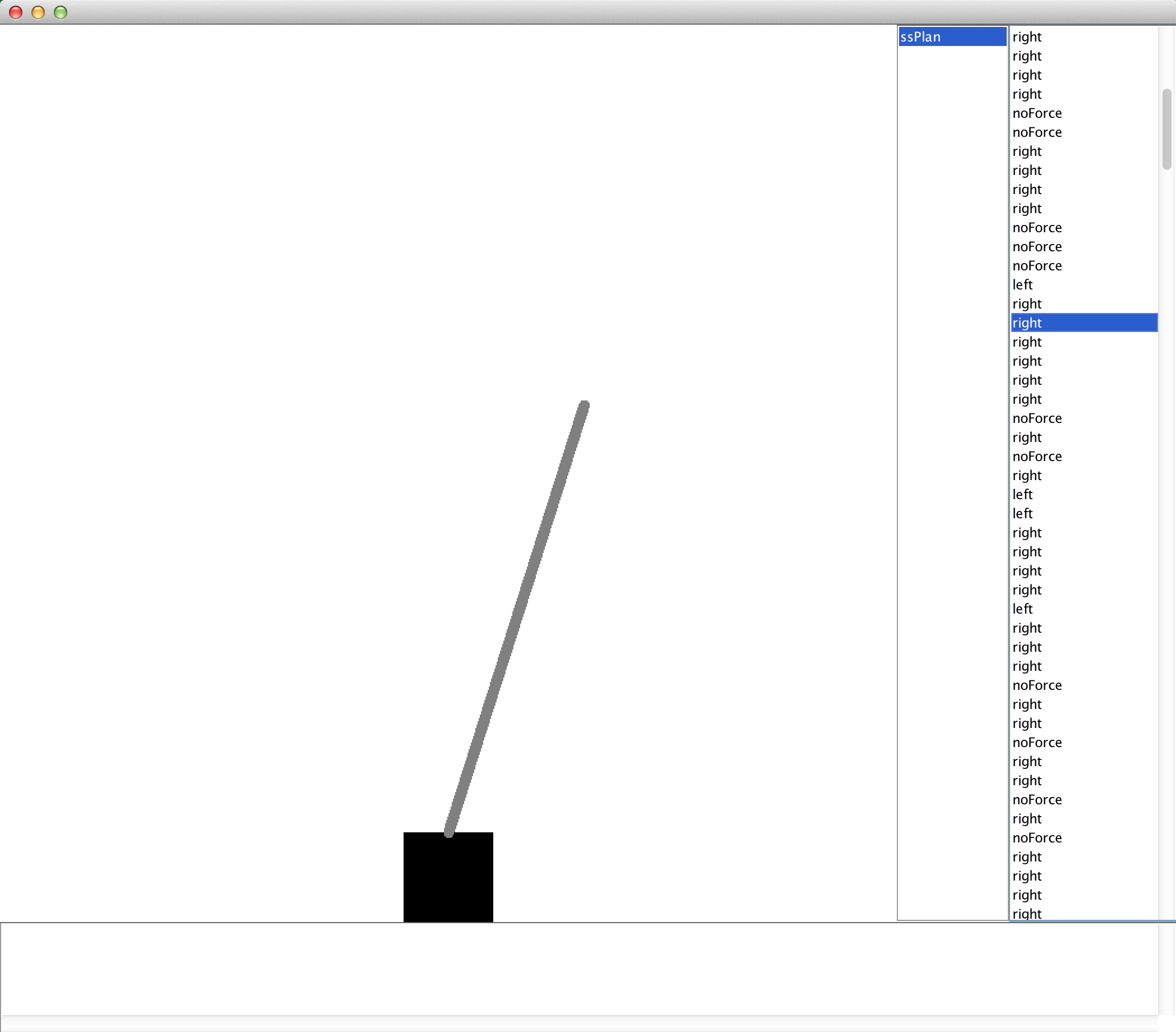
The EpisodeSequenceVisualizer GUI after solving the Inverted Pendulum with Sparse Sampling.

We're now finished with the Sparse Sampling example! If you're looking for an additional exercise, consider trying to solve this problem with LSPI using what you learned from the previous part of the tutorial. If you do so, we recommend using 5th order Fourier basis functions and collecting 5000 SARS instances by performing random trajectories from the initial balanced state. (To create a StateGenerator that always returns the same initial state for use with the SARS collector, see the ConstantStateGenerator class.)

In the final part of this tutorial, we will show how to solve the Lunar Lander domain with gradient descent SARSA lambda.

Next Part