Tutorial: Solving Continuous Domains

Tutorials (v1) > Solving Continuous Domains > Part 1

You are viewing the tutorial for BURLAP 1; if you'd like the BURLAP 2 tutorial, go here.

Introduction

In the Basic Planning and Learning tutorial we walked through how to use a number of different planning and learning algorithms. However, all the algorithms we covered were exclusively for finite state planning/learning problems and it is not uncommon in real world problems to have to deal with an infinite or continuous state space. Continuous state problems are challenging because there is an infinite number of possible states, which means you're unlikely to ever visit the same state twice. Since many of the previous algorithms rely on being ably to exhaustively enumerate the states or revisit them multiple times to estimate a value function for each state, having an infinite number of states presents a problem that requires a different set of algorithms. For example, methods that generalize the value function to unseen "near by" states is one approach to handling continuous state space problems.

In this tutorial, we will explain how to solve continuous domains, using the example domains Mountain Car, Inverted Pendulum, and Lunar Lander, with three different algorithms implemented in BURLAP that are capable of handling continuous domains: Least-Squares Policy Iteration, Sparse Sampling, and Gradient Descent Sarsa Lambda.

As usual, if you would like to see all the finished code that we will write in this tutorial, you can jump to the Final Code section at the end.

Solving Mountain Car with Least-Squares Policy Iteration

The Mountain Car domain is a classic continuous state RL domain in which an under-powered car must drive up a steep mountain. However, because the mountain is so steep, the car cannot just accelerate straight up to the top. Since car is in valley, it can, however, make it to its destination by first moving backwards up the opposite slope, and then accelerate down to gain enough momentum to get up the intended slope.

An illustration of the Mountain Car problem, courtesy of Wikipedia.

To solve this problem, we will use Least-Squares Policy Iteration (LSPI). LSPI requires a collection of state-action-reward-state (SARS) transition tuples that are sampled from the domain. In some domains, like Mountain car, this data can be collected rather straight forwardly with random sampling of actions in the world. In other domains, the set of SARS data (and therefore how it is collected) is critical to getting good results out of LSPI, so it is important to keep that in mind.

LSPI starts by initializing with a random policy and then uses the collected SARS samples to approximate the Q-value function of that policy for the continuous state space. Afterwards, the policy is updated by choosing actions that have the highest Q-values (this change in policy is known as policy improvement). This process repeats until the approximate Q-value function (and consequentially the policy) stops changing much.

LSPI approximates the Q-value function for its current policy by fitting a linear function of state basis features to the SARS data it collected, similar to a typical regression problem, which is what enables the value function to generalize to unseen states. Choosing a good set of state basis functions that can be used to accurately represent the value function is also critical to getting good performance out of LSPI. In this tutorial, we will show you how to set up Fourier basis functions and radial basis functions, which tend to be good starting places.

Lets start coding now. We'll begin by making a class shell, called ContinuousDomainTutorial. In it, we will create a different static method that demonstrates solving each domain and algorithm in this tutorial, so we'll start with our method for solving Mountain Car with LSPI using Fourier basis functions (MCLSPIFB).

public class ContinuousDomainTutorial {

	public static void main(String [] args){
		MCLSPIFB();
	}


	public static void MCLSPIFB(){
		//we'll fill this in in a moment...
	}

}
				

Next we'll create an instance of the Mountain car domain and the typical reward function and terminal function that defines the task in our MCLSPIFB method. We'll also need to add the requisite imports for this code.

import burlap.behavior.singleagent.learning.GoalBasedRF;
import burlap.domain.singleagent.mountaincar.MountainCar;
import burlap.oomdp.core.Domain;
import burlap.oomdp.core.TerminalFunction;
import burlap.oomdp.singleagent.RewardFunction;
				

MountainCar mcGen = new MountainCar();
Domain domain = mcGen.generateDomain();
TerminalFunction tf = new MountainCar.ClassicMCTF();
RewardFunction rf = new GoalBasedRF(tf, 100);
				

Our MountainCar instance provides us a means to get a TerminalFunction that sets states in which the car is on the top of the slope on the right-side as terminal states. We then define a Goal-based reward function that returns a reward of 100 when the agent reaches the terminal state and 0 everywhere else (0 is the default reward for a GoalBasedRF, but that value can be changed with a different constructor).

The next thing we will want to do is collect SARS data from the Mountain Car domain for LSPI to use for fitting its linear function approximator. For Mountain car, it is sufficient to randomly draw a state from the Mountain Car state space, sample a trajectory from it by selecting actions uniformly randomly, and then repeat the process over again from another random state. Lets collect data in this way until we have 5000 SARS tuple instances for our dataset. To accomplish this data collection, we can make use of a random StateGenerator to select random initial states, and perform random trajectory roll outs from them using a UniformRandomSARSCollector. Lets add code and the imports for that now.

import burlap.behavior.singleagent.learning.lspi.SARSCollector;
import burlap.behavior.singleagent.learning.lspi.SARSData;
import burlap.domain.singleagent.mountaincar.MCRandomStateGenerator;
import burlap.oomdp.auxiliary.StateGenerator;
				

StateGenerator rStateGen = new MCRandomStateGenerator(domain);
SARSCollector collector = new SARSCollector.UniformRandomSARSCollector(domain);
SARSData dataset = collector.collectNInstances(rStateGen, rf, 5000, 20, tf, null);
				

The MCRandomStateGenerator class provides a means to generate Mountain Car states with random positions and velocities. The collectNInstances methods will collect our SARS data for us. Specifically, we've told it to perform rollouts from states generated from our Mountain Car state generator for no more than 20 steps at a time or until we hit a terminal state. This processing a generating a random state, rolling out a random trajectory for it, and collecting all the observed SARS tuples repeats until we have 5000 SARS instances. The null parameter at the end of the method call means we want it to create a new SARSData instance and fill it up with the results (and return it) rather than adding to an existing SARSData instance.

The next thing we will want to define is the state basis features LSPI will use for its linear estimator of the value function. As noted previously, we will use Fourier basis functions. Fourier basis functions are very easy to implement without having to set many parameters, which makes it a good first approach to try.

Each Fourier basis function takes as input a feature vector defining the state, where each attribute is normalized, and produces scalar value. Each basis function corresponds to a state feature that LSPI will use for its linear function. The BURLAP FourierBasis class is an implementation of the FeatureDatabase interface and will automatically make multiple Fourier basis functions based on the order you choose. The larger the order, the more basis functions (which grow exponentially with the dimension of input state feature vector) and the more granular the representation becomes, allowing for a more precise linear value function approximation.

Recall that BURLAP states are not defined with feature vectors, but with sets of objects (adhering to the OO-MDP paradigm); however, we can convert an OO-MDP state into a feature vector trivially since OO-MDPs tend to provide more information than a standard feature vector definition does. The simplest way to convert an OO-MDP state into a feature vector is to simply concatenate the feature vector of each object in the state into a single large feature vector. To do so, we can make use of the ConcatenatedObjectFeatureVectorGenerator, which asks for which object classes to concatenate (and their concatenation order) and whether to normalize the values or not (which for Fourier basis functions we will want to do).

In the Mountain Car domain, there is only one object class—the agent—which defines the car's position and velocity, so we only need to tell the ConcatenatedObjectFeatureVectorGenerator to use the "agent" class values and to normalize its attribute values. With a feature vector conversion method in hand, lets create a set of 4th order Fourier basis functions to use as our state features for LSPI.

import burlap.behavior.singleagent.vfa.common.ConcatenatedObjectFeatureVectorGenerator;
import burlap.behavior.singleagent.vfa.fourier.FourierBasis;
				

ConcatenatedObjectFeatureVectorGenerator featureVectorGenerator = 
               new ConcatenatedObjectFeatureVectorGenerator(true, MountainCar.CLASSAGENT);

FourierBasis fb = new FourierBasis(featureVectorGenerator, 4);
				

Note that the "true" parameter in the ConcatenatedObjectFeatureVectorGenerator constructor tells it that all dimensions should be normalized in the returned feature vector, which is what Fourier basis functions expect.

Now lets instantiate LSPI on our Mountain Car domain and task with our Fourier basis functions; tell it to use a 0.99 discount factor; set its SARS dataset to the dataset we collected; and run LSPI until the weight values of its fitted linear function change no more than 10^-6 between iterations or until 30 iterations have passed.

import burlap.behavior.singleagent.learning.lspi.LSPI;
				

LSPI lspi = new LSPI(domain, rf, tf, 0.99, fb);
lspi.setDataset(dataset);

lspi.runPolicyIteration(30, 1e-6);
				

After LSPI has run until convergence, we will want to analyze the policy is produced. Since LSPI implements QComputablePlanner (which means it can return Q-values for state-action pairs), we can capture its policy by creating GreedyQ policy around it. To analyze the resulting policy, lets evaluate it from a start state in the bottom of the valley and animate the results (say 5 times). To visualize the animated results, we can simply grab the existing visualizer from the domain (MountainCarVisualizer), add a VisualActionObserver to the domain, and evaluate the policy from a start state. The state state in the valley can be retrieved from our Mountain Car domain generator instance. The code to do all that is provided below.

import burlap.behavior.singleagent.planning.commonpolicies.GreedyQPolicy;
import burlap.domain.singleagent.mountaincar.MountainCarVisualizer;
import burlap.oomdp.singleagent.SADomain;
import burlap.oomdp.core.State;
import burlap.oomdp.singleagent.common.VisualActionObserver;
import burlap.oomdp.visualizer.Visualizer;
				

GreedyQPolicy p = new GreedyQPolicy(lspi);

Visualizer v = MountainCarVisualizer.getVisualizer(mcGen);
VisualActionObserver vexp = new VisualActionObserver(domain, v);
vexp.initGUI();
((SADomain)domain).addActionObserverForAllAction(vexp);

State s = mcGen.getCleanState(domain);
for(int i = 0; i < 5; i++){
	p.evaluateBehavior(s, rf, tf);
}

System.out.println("Finished.");
				

If you now run the main method, you see at the start a bunch of print outs to the terminal specifying the maximum change in weight values after each policy iteration. When the change is small enough, LSPI will end and you'll get a window animating the the mountain car task using the results of LSPI. That is, you should see something like the below image.

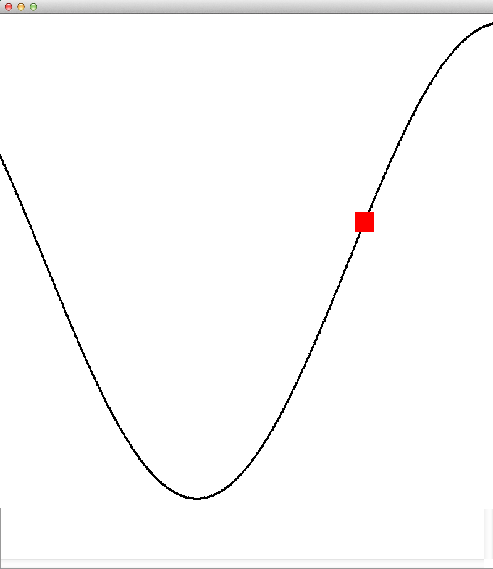
A screen cap from the animation of the Mountain car task

Although the settings we used are pretty robust to failure, it is possible (even if unlikely) that the car won't make it to the right side, which indicates that LSPI failed to find a good policy from the valley of the hill. LSPI can fail if your dataset collection happened to be unluckily bad. However, if you rerun the code (resulting in a a new random data collection), you should find that it works.

Radial Basis Functions

Before we leave Mountain Car and LSPI for the next example, lets consider running LSPI on Mountain Car with a different kind of state basis features; specifically, lets consider using radial basis functions. A radial basis function is defined with a "center" state, a distance metric, and a bandwidth parameter. Given an input query state, the basis function returns a value between 0 and 1 with a value of 1 when the query state has a distance of zero from the function's "center" state. As the query state gets further away, the basis function's returned value degrades to a value of zero. The sensitivity of the basis function to the distance is defined by its bandwidth parameter; as the bandwidth value increases, the less sensitive the function is to distance (that is, a large bandwidth will result in it returning a value near 1 even when the query state is far away).

A set of state features defined by a set of radial basis functions distributed across the state space gives an approximation of where a given state is. You can think of the set of radial basis function outputs as compressing the state space. As a consequence, a common approach to using radial basis functions is set up a coarse multi-dimensional grid over the state space with a separate radial basis function centered at each intersection point of the grid. BURLAP provides us tools to easily accomplish such a construction of radial basis functions.

Lets start by a creating a new method for running LSPI with radial basis functions. It will look almost identical to the previous Fourier Basis LSPI method we created, except instead of defining Fourier basis functions, we'll define radial basis functions. For the moment, the code below will create in instance of a radial basis function state feature database (RBFFeatureDatabase), but we will need to add code to actually add the set of radial basis functions it uses. Also note that we moved the initial state object instantiation to earlier in the code, because we will use it to help define the center states of the radial basis functions we will create. The differences are highlighted with comments in the code.

import burlap.behavior.singleagent.vfa.rbf.RBFFeatureDatabase;
				

public static void MCLSPIRBF(){

	MountainCar mcGen = new MountainCar();
	Domain domain = mcGen.generateDomain();
	TerminalFunction tf = new MountainCar.ClassicMCTF();
	RewardFunction rf = new GoalBasedRF(tf, 100);

	//get a state definition earlier, we'll use it soon.
	State s = mcGen.getCleanState(domain);

	StateGenerator rStateGen = new MCRandomStateGenerator(domain);
	SARSCollector collector = new SARSCollector.UniformRandomSARSCollector(domain);
	SARSData dataset = collector.collectNInstances(rStateGen, rf, 5000, 20, tf, null);

	//instantiate an RBF feature database, we'll define it more in a moment
	RBFFeatureDatabase rbf = new RBFFeatureDatabase(true);


	//notice we pass LSPI our RBF features this time
	LSPI lspi = new LSPI(domain, rf, tf, 0.99, rbf);
	lspi.setDataset(dataset);

	lspi.runPolicyIteration(30, 1e-6);

	GreedyQPolicy p = new GreedyQPolicy(lspi);

	Visualizer v = MountainCarVisualizer.getVisualizer(mcGen);
	VisualActionObserver vexp = new VisualActionObserver(domain, v);
	vexp.initGUI();
	((SADomain)domain).addActionObserverForAllAction(vexp);


	for(int i = 0; i < 5; i++){
		p.evaluateBehavior(s, rf, tf);
	}

	System.out.println("Finished.");

}
				

You'll notice that we passed "true" to our RBFFeatureDatabase constructor. The true flag indicates that that the feature database should include a constant feature that is always on. This is typically a good idea because it provides a Q-value "y intercept" value to the linear function that will be estimated.

To construct a set of radial basis functions over a grid, we will first want to generate the states that lie at the intersection of grid points on a grid. To construct the set of states, we will make use of the StateGridder class in BURLAP. StateGridder allows you to set up arbitrarily specified grids over a state space and return the set of states that lie on the intersection points of the grid. StateGridder can even do things like include constant values for some attributes or objects (that is, attribute values that remain fixed for every state in the grid). For our current purposes, we just want a fairly simple grid that spans the full state space of Mountain Car.

To get the set of states that span a 5x5 grid over the car position and velocity attributes (for a total of 25 states), add the below code right below the instantiation of the RBFFeatureDatabase (with the requisite imports going at the top of the file, of course). If you want to know how to set up a more specific grid (e.g., an asymmetric grid like a 3x7), see the class's documentation

import burlap.behavior.singleagent.auxiliary.StateGridder;
import java.util.List;
				

RBFFeatureDatabase rbf = new RBFFeatureDatabase(true);
StateGridder gridder = new StateGridder();
gridder.gridEntireDomainSpace(domain, 5);
List<State> griddedStates = gridder.gridInputState(s);
				

Notice that the gridInputState method requires an example State object? An example state is required because it's what tells the gridder how many objects of each object class need to be gridded (and what any constant ungridded objects/values are).

Now that we have a bunch of states distributed over a uniform grid of the state space, we will want to create radial basis functions centered at each of those states. Since a radial basis function also needs a distance metric between states, let us use a Euclidean distance metric. BURLAP already has an Euclidean distance metric implementation, but it requires that a state first be converted to a feature vector, which we can again do using the ConcatenatedObjectFeatureVectorGenerator (and we will again normalize the attribute values). To instantiate the distance metric, add the below code.

import burlap.behavior.singleagent.vfa.rbf.DistanceMetric;
import burlap.behavior.singleagent.vfa.rbf.metrics.EuclideanDistance;
				

DistanceMetric metric = new EuclideanDistance(
                 new ConcatenatedObjectFeatureVectorGenerator(true, MountainCar.CLASSAGENT));
				

Now we will add a radial basis function to our RBFFeatureDatabase for each state on the grid using the Euclidean distance metric and setting the bandwidth parameter to 0.2. In particular, we will use Gaussian radial basis functions.

import burlap.behavior.singleagent.vfa.rbf.functions.GaussianRBF;
				

for(State g : griddedStates){
	rbf.addRBF(new GaussianRBF(g, metric, .2));
}
				

Our final Mountain Car LSPI radial basis function method should now look like the below.

public static void MCLSPIRBF(){

	MountainCar mcGen = new MountainCar();
	Domain domain = mcGen.generateDomain();
	TerminalFunction tf = mcGen.new ClassicMCTF();
	RewardFunction rf = new GoalBasedRF(tf, 100);

	//get a state definition earlier, we'll use it soon.
	State s = mcGen.getCleanState(domain);

	StateGenerator rStateGen = new MCRandomStateGenerator(domain);
	SARSCollector collector = new SARSCollector.UniformRandomSARSCollector(domain);
	SARSData dataset = collector.collectNInstances(rStateGen, rf, 5000, 20, tf, null);


	//set up RBF feature database
	RBFFeatureDatabase rbf = new RBFFeatureDatabase(true);
	StateGridder gridder = new StateGridder();
	gridder.gridEntireDomainSpace(domain, 5);
	List<State> griddedStates = gridder.gridInputState(s);

	DistanceMetric metric = new EuclideanDistance(
	          new ConcatenatedObjectFeatureVectorGenerator(true, MountainCar.CLASSAGENT));
	for(State g : griddedStates){
		rbf.addRBF(new GaussianRBF(g, metric, .2));
	}

	//notice we pass LSPI our RBF features this time
	LSPI lspi = new LSPI(domain, rf, tf, 0.99, rbf);
	lspi.setDataset(dataset);

	lspi.runPolicyIteration(30, 1e-6);

	GreedyQPolicy p = new GreedyQPolicy(lspi);

	Visualizer v = MountainCarVisualizer.getVisualizer(mcGen);
	VisualActionObserver vexp = new VisualActionObserver(domain, v);
	vexp.initGUI();
	((SADomain)domain).addActionObserverForAllAction(vexp);


	for(int i = 0; i < 5; i++){
		p.evaluateBehavior(s, rf, tf);
	}

	System.out.println("Finished.");

}
				

If you now point your main method to call the MCLSPIRBF method, you should see similar results as before, only this time we've used radial basis functions!

Now that we've demonstrated how to use LSPI on the mountain car domain with Fourier basis functions and radial basis functions, we'll move on to a different algorithm, Sparse Sampling, and a different domain, the Inverted Pendulum.