Tutorial: Basic Planning and Learning
Tutorials > Basic Planning and Learning > Part 3
- Introduction
- Creating the class shell
- Initializing the data members
- Setting up a result visualizer
- Planning with BFS
- Planning with DFS
- Planning with A*
- Planning with Value Iteration
- Learning with Q-Learning
- Learning with Sarsa(λ)
- Live Visualization
- Value Function and Policy Visualization
- Experimenter Tools and Performance Plotting
- Conclusion
Planning with BFS
One of the most basic deterministic planning algorithms is breadth-first search, which we will demonstrate first. Since we will be testing a number of different planning and learning algorithms in this tutorial, we will define a separate method for using each planning or learning algorithm and then you can simply select which one you want to try in the main method of the class. We will also pass each of these methods the output path to record its results. Lets start by defining the BFS method.
public void BFSExample(String outputPath){

	DeterministicPlanner planner = new BFS(domain, goalCondition, hashingFactory);
	Policy p = planner.planFromState(initialState);
	p.evaluateBehavior(initialState, rf, tf).writeToFile(outputPath + "bfs");

}
The first part of the method creates an instance of the BFS planning algorithm, which itself is a subclass of the DeterministicPlanner class. To instantiate BFS, it only requires a reference to the domain, the goal condition for which it should search, and the HashableStateFactory. Because BFS implements the Planner interface, planning can be initiated by calling the planFromState method and passing it the initial state form which it should plan. The planFromState method automatically returns a Policy object, which can be used to query and execute the results of the planning in simulation or in an environment.
Using non-default policies
Each Planner implementation will return a different kind of Policy from planFromState that is relevant for the results the Planner stores. However, often times, after calling the planFromState method, you can wrap a different policy than the one that is returned around your planner instance to get slightly different behavior. For example, BFS's planFromState will return an SDPlannerPolicy instance, which will return the action the planner selected for any states on its solution path; if the policy is queried for a state not on the solution path, it will throw a runtime exception. However, you might choose to wrap a DDPlannerPolicy around BFS instead of using the returned SDPlannerPolicy, it will act the same except rather than throw a runtime exception if an action selection is queried for a state not on the current solution path, it will transparently recall planFromState on the new state to get an action to return; that is, it will perform replanning.
Once you have a Policy object, you can roll out the behavior and extract the resulting episode (sequence of state-action-reward tuples) from it in simulation by calling the evaluateBehavior method. There are a few different versions of the evaluateBehavior method which take different parameters to determine the analysis and stopping criteria. In this case, however, we are passing it the initial state from which the policy should start being followed, the reward function used to assess the performance and the the termination function which specifies when the policy should stop. The method will return an EpisodeAnalysis object which will contain all of the states visited, actions taken, and rewards received when following that policy. You can investigate these individual elements of the episode if you like, but for this tutorial we're just going to save the results of this episode to a file and then use the offline visualizer we previously defined to view it. An EpisodeAnalysis object can be written to a file by calling the writeToFile method on it and passing it a path to the file. Note that the method will automatically append a '.episode' extension to the file path if you did not specify it yourself and will create any directories in the path that do not already exist.
Executing policies in environments
The evaluateBehavior method can also take as input an Environment rather than a State. When given an environment, the policy is followed in the environment rather than simulation (unless of course the environment is a simulation itself!). This is very useful if you need to run planning in a model of the world, and then execute the results of that plan on something "real" or external from your model.
And that's all you need to code to plan with BFS on a defined domain and task!
Using the EpisodeSequenceVisualizer GUI
Now that the method to perform planning with BFS is defined, add a method call to it in your main method.
public static void main(String[] args) {


	BasicBehavior example = new BasicBehavior();
	String outputPath = "output/"; //directory to record results

	//run example
	example.BFSExample(outputPath);

	//run the visualizer
	example.visualize(outputPath);

}
Note that our output path ended with a '/'. Whatever path you use, you should include the trailing '/' since the code we wrote to write the file will automatically append to that path name.
With the planning method hooked up, run the code! Because the task is simple, BFS should find a solution very quickly and print to the standard output the number of nodes it expanded in its search. Following that, the GUI should be launched for viewing the EpisodeAnalysis object that was recorded to a file. You should see something like the below image appear.
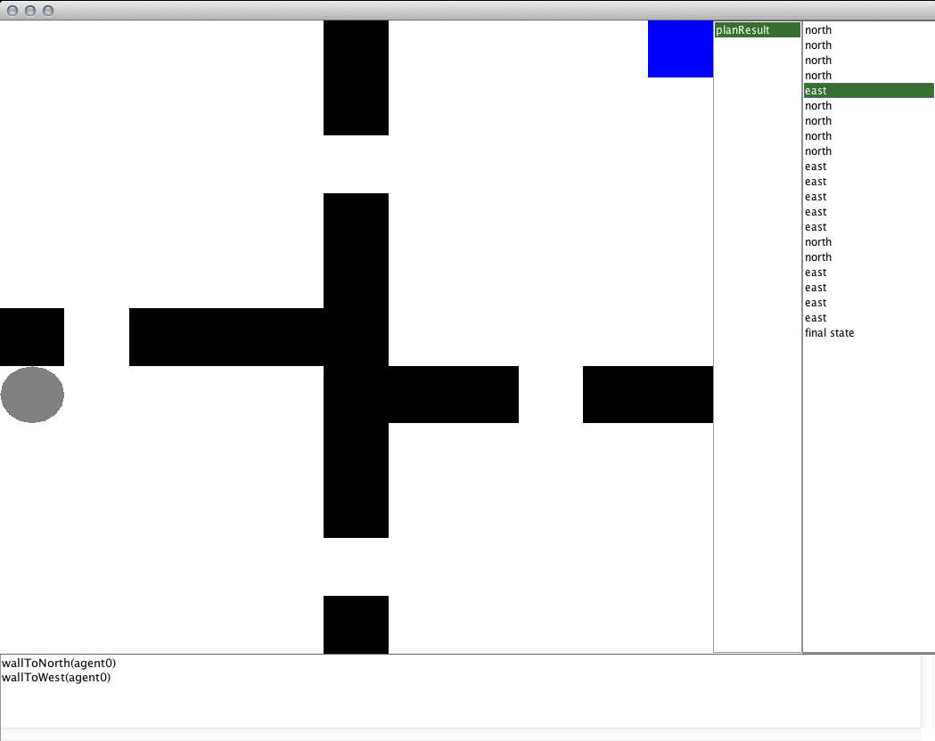
The main panel in the center of the window is used to render the current state selected. The text box at the bottom of the window will list all of the propositional functions that are true in that state. The leftmost list on the right side of the window lists all of the episode files that were recorded in the directory passed to the EpisodeSequenceVisualizer constructor. After selecting one of those instances, the list of actions taken in the episode are listed on the right-most list. Note that the action corresponds to the action that will be taken in the state that is currently visualized, so the result of the action will be seen in the next state. In the GridWorldDomain visualizer, the black cells represent walls, the grey circle represents the agent, and the blue cell represents the location object that we made.
Planning with DFS
Another common search-based planning algorithm is depth-first search (DFS). Define the below method to provide a means to solve the task with DFS.
public void DFSExample(String outputPath){

	DeterministicPlanner planner = new DFS(domain, goalCondition, hashingFactory);
	Policy p = planner.planFromState(initialState);
	p.evaluateBehavior(initialState, rf, tf).writeToFile(outputPath + "dfs");

}
You will notice that the code for DFS is effectively identical to the previous BFS code that we wrote, only this time the DeterministicPlanner is instantiated with a DFS object instead of a BFS object. DFS has a number of other constructors that allow you to specify other parameters such a depth limit, or maintaining a closed list. Feel free to experiment with them.
After you have defined the method, you can call it from the main method like we did the BFS method and visualize the results in the same way. Since DFS is not an optimal planner, it is likely that the solution it gives you will be much worse than the one BFS gave you!
Planning with A*
One of the most well known optimal search-based planning algorithms is A*. A* is an informed planner because it takes as input an admissible heuristic which estimates the cost to the goal from any given state. We can also use A* to plan a solution for our task as long as we also take the additional step of defining a heuristic to use (or you can use a NullHeuristic which will make A* uninformed). The below code defines a method for using A* with a Manhattan distance to goal heuristic.
public void AStarExample(String outputPath){

	Heuristic mdistHeuristic = new Heuristic() {
		@Override
		public double h(State s) {

			ObjectInstance agent = s.getFirstObjectOfClass(GridWorldDomain.CLASSAGENT);
			ObjectInstance location = s.getFirstObjectOfClass(GridWorldDomain.CLASSLOCATION);

			int ax = agent.getIntValForAttribute(GridWorldDomain.ATTX);
			int ay = agent.getIntValForAttribute(GridWorldDomain.ATTY);

			int lx = location.getIntValForAttribute(GridWorldDomain.ATTX);
			int ly = location.getIntValForAttribute(GridWorldDomain.ATTY);

			double mdist = Math.abs(ax-lx) + Math.abs(ay-ly);
			return -mdist;
		}
	};

	DeterministicPlanner planner = new AStar(domain, rf, goalCondition,
											hashingFactory, mdistHeuristic);
	Policy p = planner.planFromState(initialState);
	p.evaluateBehavior(initialState, rf, tf).writeToFile(outputPath + "astar");

}
There are two main differences between this method and the methods that we wrote for BFS and DFS planning. The smaller difference is that the A* constructor includes a reward function in its parameters. The reward function is needed because it is what A* uses to keep track of the actual cost of any path it is exploring.
Rewards and Costs
A* is an algorithm that operates on costs and is not an algorithm that can work with negative costs. BURLAP in general represents state-action evaluations as rewards, rather than costs. However, a cost can be represented as a negative reward; therefore, the reward function provided to A* should return negative values. If the reward function returns any positive values, A* will not function properly. Since our example's reward function returns only negative values (it returns -1 for every state-action pair), our reward function will work fine with A*.
The bigger difference between the previous planning code and A* is in defining the heuristic, which we do by implementing the Heuristic interface. The h method of the Heuristic interface is passed a state object and the method should return the estimated reward to the goal from that state (which should be a non-positive value). Since we have opted to use the Manhattan distance as our heuristic, this will involve computing the distance between the agent position and the location position (for which we will assume there is only one). To compute this difference, the method will first need to extract the agent object instance and the location object instance out of the state, which is done in lines 7 and 8. Specifically, the getFirstObjectOfClass method of a state will return the first object in the state that belongs to the OO-MDP class with the given name. Lines 10-14 then extract the integer values for the X and Y attributes of both the agent and location objects. Once those attribute values are retrieved, the Manhattan distance is computed and returned in lines 16 and 17. Note that the negative distance is returned, because our reward function returns -1 for each step.
With the rest of the code being the same, you can have the main method call the A* method for planning and view the results in the usual way!