Tutorial: Basic Planning and Learning
Tutorials > Basic Planning and Learning > Part 5
- Introduction
- Creating the class shell
- Initializing the data members
- Setting up a result visualizer
- Planning with BFS
- Planning with DFS
- Planning with A*
- Planning with Value Iteration
- Learning with Q-Learning
- Learning with Sarsa(λ)
- Live Visualization
- Value Function and Policy Visualization
- Experimenter Tools and Performance Plotting
- Conclusion
Live Visualization
Although we showed how to visualize learning or planning results after they had been performed, sometimes when setting up a new problem and experiment it is useful to watch what is happening immediately. In this part of the tutorial we show how to set up a live visualization of learning algorithms or planning algorithms that operate by trying actions in the world (more on that in a bit). To present a live visualization we make use of the ActionObserver and EnvironmentObserver interfaces. Objects that implement the ActionObserver interface can be notified about action execution results in simulation; objects that implement the EnvironmentObserver interface can be told about agent interactions with an Environment. In this example, we will instantiate a VisualActionObserver and which implements both interfaces and visualizes state changes.
The scope of ActionObserver
It is worth noting that an ActionObserver is only notifed when the performAction method of Action instances is called. This method is used by various sample based planning algorithms and detemrinistic planning algorithms. However, algorithms like VI do not use this method because they instead operate on the full action probability distribution (returned by the getTransitions method) rather than simulating actions.
To add a VisualActionObserver, we can modify our constructor by adding the following lines to then end of it:
VisualActionObserver observer = new VisualActionObserver(domain,
		GridWorldVisualizer.getVisualizer(gwdg.getMap()));
observer.initGUI();
env = new EnvironmentServer(env, observer);
//((SADomain)domain).addActionObserverForAllAction(observer);
The first line creates a VisualActionObserver for visualizing our domain with a provided domain state visualizer (we use the same kind of state visualizer that we used for our EpisodeSequenceVisualizer). The second line initializes the Java GUI for its visualization. You can then choose whether to use the third line or the commented out fourth line. The third line is how we set up the VisualActionObserver to receive events from an Environment and requires changing our Environment to an EnvironmentServer. An EnvironmentServer takes as input a source environment, and a list of EnvironmentObservers. Normal operations for the environment are delegated to the source environment, but the outcomes of the interaction are intercepted and sent to all observers before returning control to the client. The commented out fourth line would tell all the Action objects in the domain to add the action observer that is notified whenever the action is run in simulation.
If you want to test the action observer out with a learning algorithm use the EnvironmentObserver paradigm (third line). If you want to test it with one of the deterministic planners, comment out the third line and uncomment the fourth. Which ever you choose, you should find that when you run the algorithm you observe the agent moving through the environment!
Performance with VisualActionObservers
By default, the VisualActionObserver will render frames at about 60FPS. You can modify this rate with the setFrameDelay(long delay) method, which takes as an argument the number of milliseconds that must pass for the rendering of an event and before the next action can be taken. Note that this delay also places a cap on the speed at which learning or planning occurs since it stalls everything for that frame delay. Typically, learning in BURLAP occurs at speeds orders of magnitude faster than 60FPS, so using the visual observer will slow down your algorithm considerably. For these reasons, you may prefer the offline visualization. Nevertheless, live visualization is often a useful as a way to confirm that your experiment is working as planned.
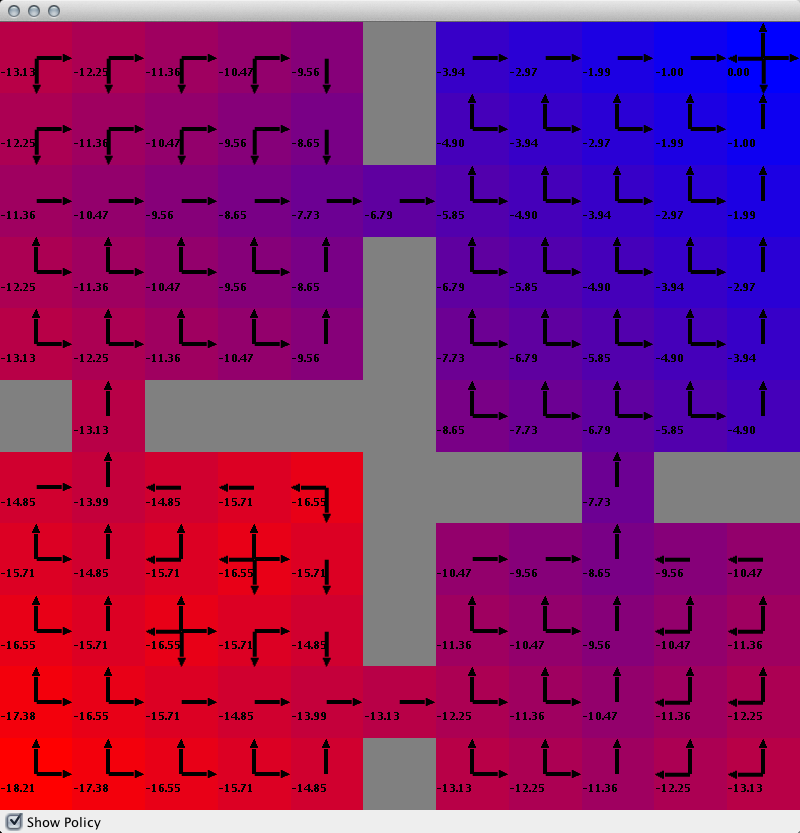
Value Function and Policy Visualization
While visualizing the agent in the state space is useful, in this next section, we will show how to visualize the value function that is estimated from value function estimating planning or learning algorithms, along with the corresponding policy. The value function assigns a value to each state that represents the expected future discounted reward when following the optimal policy from that state. In particular, we will show how to visualize the value function for the ValueIteration results, but you could do the same with Q-Learning, or any planning/learning algorithm that implements the ValueFuncton interface (which the QFunction interface extends).
We will show you how to construct a value function visualizer in two ways. In the first way, we will make use of a GridWorldDomain method that will put all the pieces together for you and is very simple. However, since not all domains have automated code for that, we will also show you how to put all the pieces together manually. Lets start with the simple way, which requires adding the following method to your code.
public void simpleValueFunctionVis(ValueFunction valueFunction, Policy p){

	List<State> allStates = StateReachability.getReachableStates(initialState,
						(SADomain)domain, hashingFactory);
	ValueFunctionVisualizerGUI gui = GridWorldDomain.getGridWorldValueFunctionVisualization(
					allStates, valueFunction, p);
	gui.initGUI();

}
Note that this method takes as input a ValueFunction instance and a Policy object (since along with the value function, we will also render the policy). Before we do anything with it, we are going to have to tell the renderer for which states we'd like to visualize the value function. Although Domain objects are not required to enumerate the entire state space (since for many domains that might be impossible), we can use the BURLAP tool StateReachability to find all states that are reachable from some input state. (Algorithms like ValueIteraiton also have a method to return all states that they enumerated that we could have used.)
Next we call the GridWorldDomain method getGridWorldValueFunctionVisualization, which takes the set of states for which the value function will be rendered, the ValueFunction instance, and the Policy to render and returns a ValueFunctionVisualizationGUI instance that will do it for us. Finally, we launch the return GUI with the initGUI method.
The last step is to direct our value iteration method to this method once planning is complete. Your new value iteration method should look like the following.
public void valueIterationExample(String outputPath){

	Planner planner = new ValueIteration(domain, rf, tf, 0.99, hashingFactory, 0.001, 100);
	Policy p = planner.planFromState(initialState);
	p.evaluateBehavior(initialState, rf, tf).writeToFile(outputPath + "vi");

	//visualize the value function and policy.
	simpleValueFunctionVis((ValueFunction)planner, p);

}
If you now point your main method to run the valueIterationExample, you should find that after planning completes, it launches a GUI like the below (note that you can toggle the policy visualization with the check box in the bottom left).
Now that we've shown you how to easily create a value function and policy visualization for grid worlds, lets walk through the process of manually creating one so that you know how to do so for other domains. Add the following method to your code.
public void manualValueFunctionVis(ValueFunction valueFunction, Policy p){

	List<State> allStates = StateReachability.getReachableStates(initialState,
						(SADomain)domain, hashingFactory);

	//define color function
	LandmarkColorBlendInterpolation rb = new LandmarkColorBlendInterpolation();
	rb.addNextLandMark(0., Color.RED);
	rb.addNextLandMark(1., Color.BLUE);

	//define a 2D painter of state values, specifying which attributes correspond
	//to the x and y coordinates of the canvas
	StateValuePainter2D svp = new StateValuePainter2D(rb);
	svp.setXYAttByObjectClass(GridWorldDomain.CLASSAGENT, GridWorldDomain.ATTX,
			GridWorldDomain.CLASSAGENT, GridWorldDomain.ATTY);

	//create our ValueFunctionVisualizer that paints for all states
	//using the ValueFunction source and the state value painter we defined
	ValueFunctionVisualizerGUI gui = new ValueFunctionVisualizerGUI(allStates, svp, valueFunction);

	//define a policy painter that uses arrow glyphs for each of the grid world actions
	PolicyGlyphPainter2D spp = new PolicyGlyphPainter2D();
	spp.setXYAttByObjectClass(GridWorldDomain.CLASSAGENT, GridWorldDomain.ATTX,
			GridWorldDomain.CLASSAGENT, GridWorldDomain.ATTY);
	spp.setActionNameGlyphPainter(GridWorldDomain.ACTIONNORTH, new ArrowActionGlyph(0));
	spp.setActionNameGlyphPainter(GridWorldDomain.ACTIONSOUTH, new ArrowActionGlyph(1));
	spp.setActionNameGlyphPainter(GridWorldDomain.ACTIONEAST, new ArrowActionGlyph(2));
	spp.setActionNameGlyphPainter(GridWorldDomain.ACTIONWEST, new ArrowActionGlyph(3));
	spp.setRenderStyle(PolicyGlyphPainter2D.PolicyGlyphRenderStyle.DISTSCALED);

	//add our policy renderer to it
	gui.setSpp(spp);
	gui.setPolicy(p);

	//set the background color for places where states are not rendered to grey
	gui.setBgColor(Color.GRAY);

	//start it
	gui.initGUI();


}
The method signature looks the same as before and also as before we will use StateReachability to get all the states for which the value function will be rendered. Since we will be rendering the value of a cell of the grid world with a color that blends from red to blue, we will create an instance of the ColorBlend interface. In particular, we will use the LandmarkColorBlendInterpolation. This class lets you input a real value that spits out a color that is interpolated between various specified colors. So in this case, we defined the interpolation to blend from red to blue (we could have added additional points of color in between; feel free to experiment). The numeric values to which we assign these colors are normalized, so 0 is the minimum value and 1 is the maximum.
Next we want to define a StateValuePainter instance, which is an interface that has a method that takes as input a graphics context, a State and a value for that state and renders it to the graphics context. In particular, we will use the StateValuePainter2D implementation, which will rendered colored cells for each state where the color to render is based on a ColorBlend instance (which we defined above). For this class to determine where in a graphics context to render a state's cell, it needs to be told what object class and attributes in the state represent the x and y position in the 2D world. So in this case, we tell it to use the agent's x and y positions.
At this point, we create our ValueFunctionVisualizerGUI instance, which takes the states for which to render the value, the StateValuePainter to use, and the source ValueFunction that specifies the value for the states. However, before we finish, we also added a Policy renderer that can overlay the value function visualization. For this rendering, we will need a StatePolicyPainter implementation and in the code we use a PolicyGlyphPainter2D that renders a policy at some position in a 2D graphics context by drawing glyphs for the selected action (or actions if there are a set of actions that the policy selects). Like the StateValuePainter2D, this class needs to be told what the object class attributes in a State indicate the 2D position in the graphics context. It also needs to be told which ActionGlyphPainterto use to paint a glyph for each action (by action name). Here we used the existing ArrowActionGlyph for each action, where the parameter in its constructor for 0 to 3 indicates a north, south east, and west arrow respectively. The PolicyGlyphPainter2D also have various ways to render the glyphs. Here we use DISTSCALED which means each action glyph is rendered at a size proportional to the probability that the agent will select that action.
Finally, we set the ValueFunctionVisualizerGUI to use the StatePolicyPainter we created, and set the Policy it should render. Then we set the background color to gray, and launch the GUI. If you now point the value iteration method to this value function visualization method instead of the simple one, you should find that your get the same visualization.